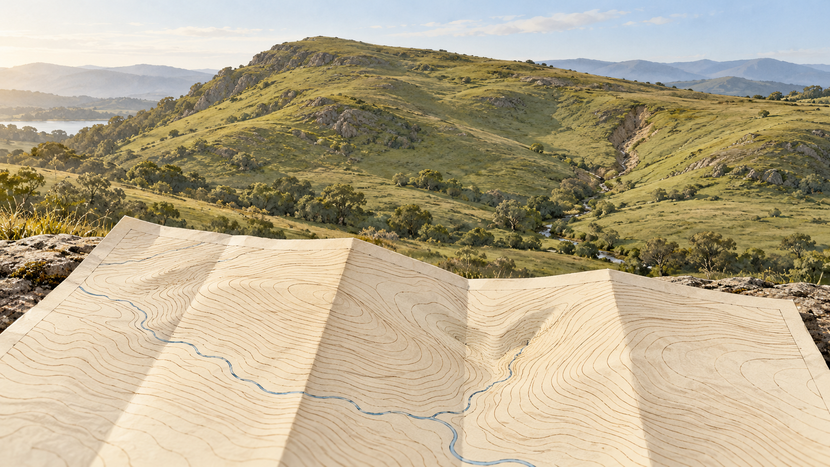
A contour line makes a precise-looking promise: every point along it has the same mapped height. The line is imaginary on the ground, yet it gives a flat sheet the shape of a hill. The intervals between lines require more care. A map can tell us that a slope rises from one selected elevation to the next. It cannot show every stone, hollow or change of grade that fits in that space. The useful skill is to read what the curves support, then recognize the ground they have left for us to infer.
A series of level slices
Imagine a hillside meeting a succession of level water surfaces. The edge where each surface touches the land would draw a contour. A topographic map chooses those levels at a regular vertical separation, called the contour interval. On one Ordnance Survey map that separation might be five metres; on another, ten. Its relief and contours guide shows both intervals at different map scales. The number belongs to the particular map, not to the landscape. A reader should find it before converting the pattern into a mental picture of a climb.
When contours crowd together, the land gains or loses the same vertical interval over a short horizontal distance. It is steep there. When they spread apart, that change takes more ground distance and the broad slope is gentler. The Ordnance Survey guide illustrates valleys, a saddle and cliffs as different patterns of lines. A loop enclosing higher contours may suggest a hill; a narrow neck between high ground may suggest a pass. Those patterns are powerful because several lines make a form visible. A single curve says only that the model has reached one elevation along that path.
Even the simplest estimate between two adjacent lines assumes something. Halfway across the space on paper is tempting to read as halfway up in height. That will be close only if the slope changes fairly evenly across that section. A bench near the lower line followed by a sharp rise near the upper one would give the same two contours but a different height at the midpoint. The lines bound an elevation range; they do not specify a straight ramp between themselves. A steep patch may also sit within a generally gentle slope without commanding its own contour if it does not cross another chosen level.
The small shape that does not earn a line
Now imagine a shallow hollow whose rim and floor both fall between two contour elevations. Neither selected level cuts through it. The map may show a smooth hillside where a walker finds a dip, a wet pocket or a short steep bank. This is a consequence of sampling height at intervals, not necessarily a mistake by a mapmaker. The smaller the feature relative to the interval and the map scale, the easier it is to omit or generalize. A US Geological Survey study of closed depressions makes the practical problem sharper: both source elevation data and interpolation into a grid can create false hollows or conceal real ones. Its investigators used field visits as part of separating likely depressions from artifacts. The study concerns karst terrain in parts of the southeastern United States; it is evidence for the need to verify consequential small features, not a claim that every blank patch hides a sinkhole.
The opposite mistake is possible too. A closed curve on a digital surface can look like a basin even when an unmodeled culvert or bridge carries water through the apparent barrier. The USGS lidar specification requires a logical interpolated bare-earth surface beneath bridges and particular treatments for water surfaces. Those choices help a map behave as terrain rather than as a literal record of every elevated structure. They also remind us that a contour is drawn from a model of the ground. It is not a pencil tracing of an unmediated scan.
How the curves reach the page
Modern elevation maps commonly begin with measured points and a digital elevation model, then draw lines through selected heights. The USGS 3D Elevation Program description explains that lidar and, in Alaska, radar-derived elevation data feed bare-earth models and that derived contours appear on US Topo maps. More observations can resolve more small terrain, but point density and vertical accuracy are separate properties. A closely sampled surface can still carry errors in the height assigned to its points, and a beautifully smooth line can disguise gaps or a poor source model.
Turning a raw digital line into a readable map adds another stage. In an original USGS study of digital contour production, cartographers found that automatically generated contours needed smoothing and checks against mapped water features. Imperfect elevation grids and the work of reconciling the lines with streams caused practical difficulties. Smoothing is useful: without it, little artifacts in a grid can make a contour shake and distract from the landform. But it means the exact wiggle of a printed curve is not always an independent observation of a wiggle in the hillside. Its shape has passed through measurement, interpolation and drawing rules.
The map itself can disclose some of that history. The USGS guide to US Topo maps says each map file includes metadata describing its data sources and production process. US Topo sheets also combine contours with imagery, hydrography and shaded relief. When a critical detail seems absent or contradictory, the date and source of the elevation layer matter more than how sharply the PDF can be enlarged. Zooming makes the line bigger; it does not measure the missing hillside.
These limits do not make contours untrustworthy. They make them a particular kind of evidence. For an overall route, a drainage divide or the broad side of a valley, the repeated curves quickly convey form. For the exact position of a small channel, the grade at a building site or a shallow closed hollow, the interval, data source, mapping process and an observation on the ground may all matter. The space between two curves is where the map stops speaking in measured levels and the reader begins to reason. Good map reading keeps that boundary visible.
A thought worth keeping?